Graphene hv scan

Simple workflow for analyzing a photon energy scan data of graphene as simulated from a third nearest neighbor tight binding model. The same workflow can be applied to any photon energy scan.

Import the “fundamental” python libraries for a generic data analysis:

import numpy as np
import matplotlib.pyplot as plt

Instead of loading the file as for example:

# from navarp.utils import navfile
# file_name = r"nxarpes_simulated_cone.nxs"
# entry = navfile.load(file_name)

Here we build the simulated graphene signal with a dedicated function defined just for this purpose:

from navarp.extras.simulation import get_tbgraphene_hv

entry = get_tbgraphene_hv(
    scans=np.arange(90, 150, 2),
    angles=np.linspace(-7, 7, 300),
    ebins=np.linspace(-3.3, 0.4, 450),
    tht_an=-18,
)

Plot a single analyzer image at scan = 90

First I have to extract the isoscan from the entry, so I use the isoscan method of entry:

iso0 = entry.isoscan(scan=90)

Then to plot it using the ‘show’ method of the extracted iso0:

iso0.show(yname='ekin')

Out:

<matplotlib.collections.QuadMesh object at 0x7fc56da82350>

Or by string concatenation, directly as:

entry.isoscan(scan=90).show(yname='ekin')

Out:

<matplotlib.collections.QuadMesh object at 0x7fc570ac4bd0>

Fermi level determination

The initial guess for the binding energy is: ebins = ekins - (hv - work_fun). However, the better way is to proper set the Fermi level first and then derives everything form it. In this case the Fermi level kinetic energy is changing along the scan since it is a photon energy scan. So to set the Fermi level I have to give an array of values corresponding to each photon energy. By definition I can give:

efermis = entry.hv - entry.analyzer.work_fun
entry.set_efermi(efermis)

Or I can use a method for its detection, but in this case, it is important to give a proper energy range for each photon energy. For example for each photon a good range is within 0.4 eV around the photon energy minus the analyzer work function:

energy_range = (
    (entry.hv[:, None] - entry.analyzer.work_fun) +
    np.array([-0.4, 0.4])[None, :])

entry.autoset_efermi(energy_range=energy_range)

Out:

scan(eV)  efermi(eV)  FWHM(meV)  new hv(eV)
90.0000  85.4000  58.8  90.0000
92.0000  87.4003  58.6  92.0003
94.0000  89.4002  58.1  94.0002
96.0000  91.4002  58.7  96.0002
98.0000  93.4000  59.2  98.0000
100.0000  95.4003  58.4  100.0003
102.0000  97.4006  58.3  102.0006
104.0000  99.4010  56.6  104.0010
106.0000  101.3999  59.4  105.9999
108.0000  103.4004  58.7  108.0004
110.0000  105.4006  57.6  110.0006
112.0000  107.4003  58.5  112.0003
114.0000  109.4003  60.6  114.0003
116.0000  111.3999  59.3  115.9999
118.0000  113.3998  60.0  117.9998
120.0000  115.4002  59.4  120.0002
122.0000  117.4005  58.2  122.0005
124.0000  119.4002  59.3  124.0002
126.0000  121.4009  58.6  126.0009
128.0000  123.4005  58.1  128.0005
130.0000  125.4001  59.4  130.0001
132.0000  127.4006  57.4  132.0006
134.0000  129.4000  59.7  134.0000
136.0000  131.4003  58.2  136.0003
138.0000  133.3999  58.9  137.9999
140.0000  135.4004  58.6  140.0004
142.0000  137.3998  58.7  141.9998
144.0000  139.4003  60.1  144.0003
146.0000  141.4002  59.3  146.0002
148.0000  143.4004  59.1  148.0004

In both cases the binding energy and the photon energy will be updated consistently. Note that the work function depends on the beamline or laboratory. If not specified is 4.5 eV.

To check the Fermi level detection I can have a look on each photon energy. Here I show only the first 10 photon energies:

for scan_i in range(10):
    print("hv = {} eV,  E_F = {:.0f} eV,  Res = {:.0f} meV".format(
        entry.hv[scan_i],
        entry.efermi[scan_i],
        entry.efermi_fwhm[scan_i]*1000
    ))
    entry.plt_efermi_fit(scan_i=scan_i)

• 
• 
• 
• 
• 
• 
• 
• 
• 
• 

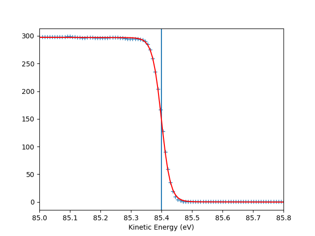
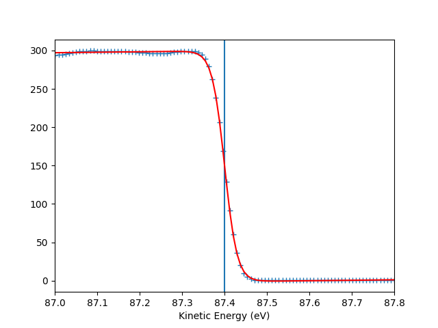
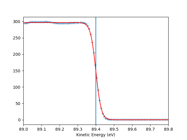
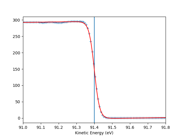
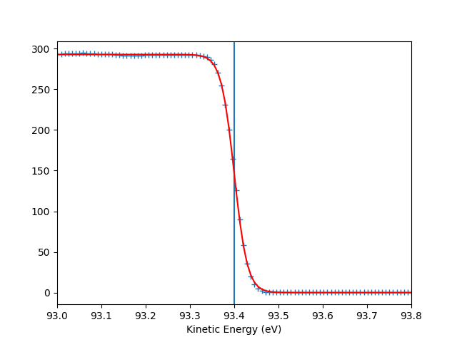
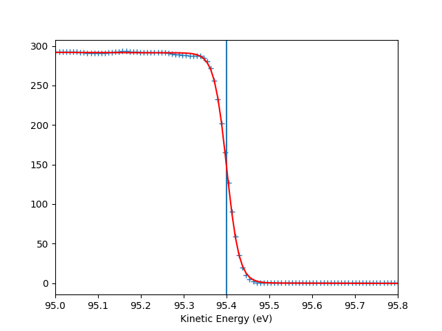
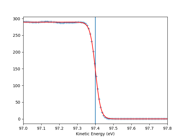
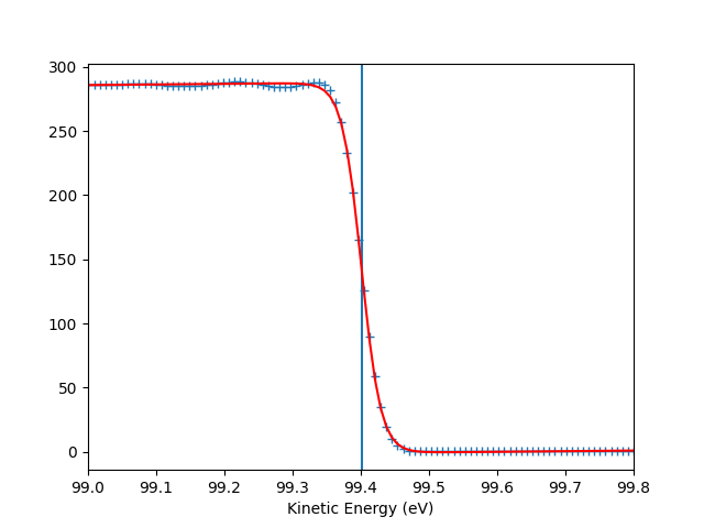
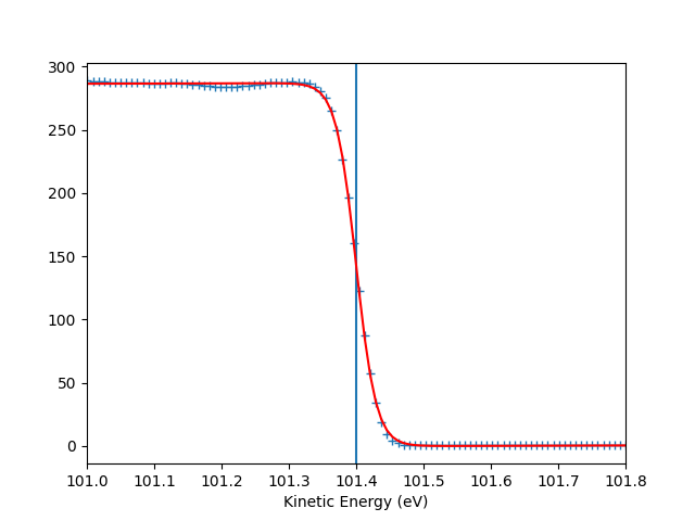
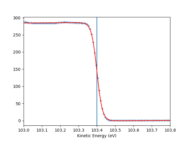
Out:

hv = 90.0000026322631 eV,  E_F = 85 eV,  Res = 59 meV
hv = 92.00034396834147 eV,  E_F = 87 eV,  Res = 59 meV
hv = 94.00020052850076 eV,  E_F = 89 eV,  Res = 58 meV
hv = 96.0002071725171 eV,  E_F = 91 eV,  Res = 59 meV
hv = 97.99996511943282 eV,  E_F = 93 eV,  Res = 59 meV
hv = 100.00033060955292 eV,  E_F = 95 eV,  Res = 58 meV
hv = 102.00057713915359 eV,  E_F = 97 eV,  Res = 58 meV
hv = 104.00101948382944 eV,  E_F = 99 eV,  Res = 57 meV
hv = 105.99986522692515 eV,  E_F = 101 eV,  Res = 59 meV
hv = 108.0004287342628 eV,  E_F = 103 eV,  Res = 59 meV

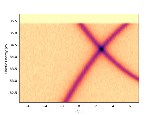
Plot a single analyzer image at scan = 110 with the Fermi level aligned

entry.isoscan(scan=110).show(yname='eef')

Out:

<matplotlib.collections.QuadMesh object at 0x7fc56d553890>

Plotting iso-energetic cut at ekin = efermi

entry.isoenergy(0).show()

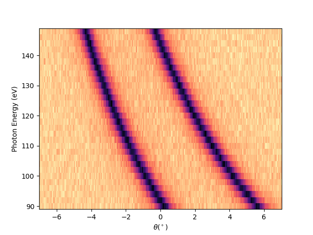
Out:

<matplotlib.collections.QuadMesh object at 0x7fc56db2c0d0>

Plotting in the reciprocal space (k-space)

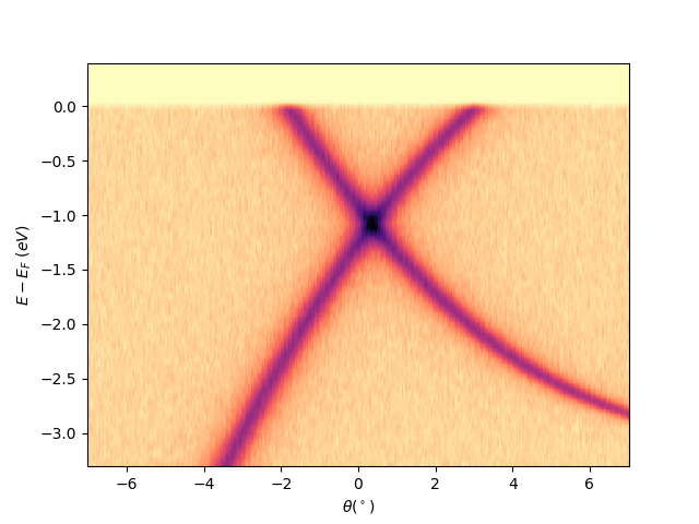
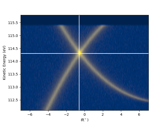
I have to define first the reference point to be used for the transformation. Meaning a point in the angular space which I know it correspond to a particular point in the k-space. In this case the graphene Dirac-point is for hv = 120 is at ekin = 114.3 eV and tht_p = -0.6 (see the figure below), which in the k-space has to correspond to kx = 1.7.

hv_p = 120

entry.isoscan(scan=hv_p, dscan=0).show(yname='ekin', cmap='cividis')

tht_p = -0.6
e_kin_p = 114.3
plt.axvline(tht_p, color='w')
plt.axhline(e_kin_p, color='w')

entry.set_kspace(
    tht_p=tht_p,
    k_along_slit_p=1.7,
    scan_p=0,
    ks_p=0,
    e_kin_p=e_kin_p,
    inn_pot=14,
    p_hv=True,
    hv_p=hv_p,
)

Out:

tht_an = -18.040
scan_type =  hv
inn_pot = 14.000
phi_an = 0.000
k_perp_slit_for_kz = 0.000
kspace transformation ready

Once it is set, all the isoscan or iscoenergy extracted from the entry will now get their proper k-space scales:

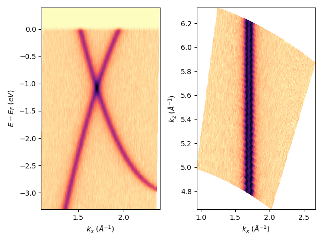
entry.isoscan(120).show()

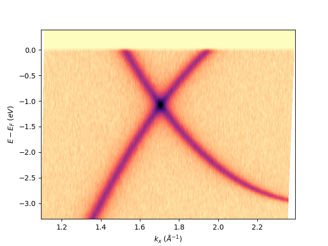
Out:

<matplotlib.collections.QuadMesh object at 0x7fc56da91f90>

sphinx_gallery_thumbnail_number = 17

entry.isoenergy(0).show(cmap='cividis')

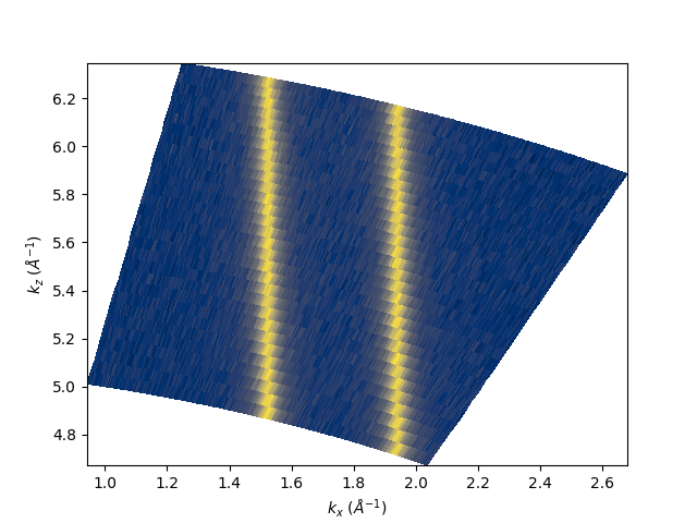
Out:

<matplotlib.collections.QuadMesh object at 0x7fc570aaf410>

I can also place together in a single figure different images:

fig, axs = plt.subplots(1, 2)

entry.isoscan(120).show(ax=axs[0])
entry.isoenergy(-0.9).show(ax=axs[1])

plt.tight_layout()

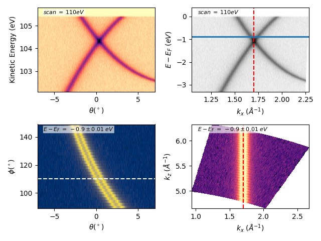
Many other options:

fig, axs = plt.subplots(2, 2)

scan = 110
dscan = 0
ebin = -0.9
debin = 0.01

entry.isoscan(scan, dscan).show(ax=axs[0][0], xname='tht', yname='ekin')
entry.isoscan(scan, dscan).show(ax=axs[0][1], cmap='binary')

axs[0][1].axhline(ebin-debin)
axs[0][1].axhline(ebin+debin)

entry.isoenergy(ebin, debin).show(
    ax=axs[1][0], xname='tht', yname='phi', cmap='cividis')
entry.isoenergy(ebin, debin).show(
    ax=axs[1][1], cmap='magma', cmapscale='log')

axs[1][0].axhline(scan, color='w', ls='--')
axs[0][1].axvline(1.7, color='r', ls='--')
axs[1][1].axvline(1.7, color='r', ls='--')

x_note = 0.05
y_note = 0.98

for ax in axs[0][:]:
    ax.annotate(
        "$scan \: = \: {} eV$".format(scan, dscan),
        (x_note, y_note),
        xycoords='axes fraction',
        size=8, rotation=0, ha="left", va="top",
        bbox=dict(
            boxstyle="round", fc='w', alpha=0.65, edgecolor='None', pad=0.05
        )
    )

for ax in axs[1][:]:
    ax.annotate(
        "$E-E_F \: = \: {} \pm {} \; eV$".format(ebin, debin),
        (x_note, y_note),
        xycoords='axes fraction',
        size=8, rotation=0, ha="left", va="top",
        bbox=dict(
            boxstyle="round", fc='w', alpha=0.65, edgecolor='None', pad=0.05
        )
    )

plt.tight_layout()